Advanced RAG 12: Enhancing Global Understanding
Priciples, Code Explanation and Insights
Many important real-world tasks, including scientific literature review, legal case briefing, and medical diagnosis, require knowledge understanding across chunks or documents.
Existing RAG methods are unable to aid LLMs in tasks that demand the comprehension of information across chunk boundaries, as each chunk is encoded independently.
This article will introduce four innovative methods to enhance the global understanding of documents or corpora, along with insights and thoughts learned from them.
The four methods are as follows:
RAPTOR: This is a tree-based retrieval system that recursively embeds, clusters, and summarizes text chunks.
Graph RAG: This method combines knowledge graph generation, community detection, RAG, and Query-Focused Summarization (QFS) to facilitate a comprehensive understanding of the entire text corpus.
HippoRAG: This retrieval framework draws inspiration from the hippocampal indexing theory of human long-term memory. It collaborates with LLMs, knowledge graphs, and personalized PageRank algorithms.
spRAG: This method enhances the performance of the standard RAG system through two key techniques, namely AutoContext and Relevant Segment Extraction (RSE).
RAPTOR: Recursive Abstractive Processing for Tree-Organized Retrieval
RAPTOR is a novel tree-based retrieval system designed for recursively embedding, clustering, and summarizing text segments. It constructs a tree from the bottom up, offering varying levels of summarization.
During inference, RAPTOR retrieves information from this tree, incorporating data from longer documents at various levels of abstraction.
Key Idea
RAPTOR employs a recursive method to organize text chunks into clusters based on their embeddings. It generates summaries for each of these clusters, constructing a tree from the bottom up. This process is illustrated in Figure 1.
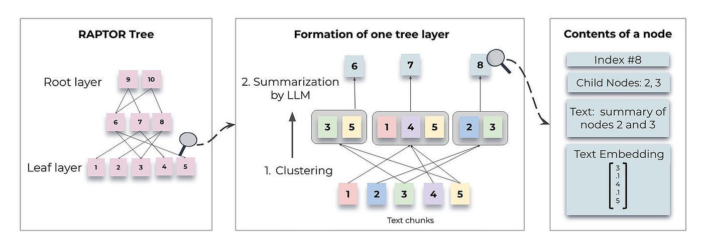
Below we delve into specific topics related to Figure 1:
Constructing a RAPTOR tree
Retrieval processes
Constructing a RAPTOR Tree
Text Chunking
Divide the retrieval corpus into continuous chunks of 100 tokens each. If a chunk exceeds 100 tokens, RAPTOR shifts the entire sentence to the next chunk to maintain contextual and semantic coherence.
def split_text(
    text: str, tokenizer: tiktoken.get_encoding("cl100k_base"), max_tokens: int, overlap: int = 0
):
    """
    Splits the input text into smaller chunks based on the tokenizer and maximum allowed tokens.

    Args:
        text (str): The text to be split.
        tokenizer (CustomTokenizer): The tokenizer to be used for splitting the text.
        max_tokens (int): The maximum allowed tokens.
        overlap (int, optional): The number of overlapping tokens between chunks. Defaults to 0.

    Returns:
        List[str]: A list of text chunks.
    """
    ...
    ...
        # If adding the sentence to the current chunk exceeds the max tokens, start a new chunk
        elif current_length + token_count > max_tokens:
            chunks.append(" ".join(current_chunk))
            current_chunk = current_chunk[-overlap:] if overlap > 0 else []
            current_length = sum(n_tokens[max(0, len(current_chunk) - overlap):len(current_chunk)])
            current_chunk.append(sentence)
            current_length += token_count
    ...
    ...
Embedding
Use Sentence-BERT to generate the dense vector representation of these chunks.
These chunks, along with their corresponding embeddings, constitute the leaf nodes of RAPTOR tree structure.
class TreeBuilder:
    """
    The TreeBuilder class is responsible for building a hierarchical text abstraction
    structure, known as a "tree," using summarization models and
    embedding models.
    """
    ...
    ...
    def build_from_text(self, text: str, use_multithreading: bool = True) -> Tree:
        """Builds a golden tree from the input text, optionally using multithreading.

        Args:
            text (str): The input text.
            use_multithreading (bool, optional): Whether to use multithreading when creating leaf nodes.
                Default: True.

        Returns:
            Tree: The golden tree structure.
        """
        chunks = split_text(text, self.tokenizer, self.max_tokens)

        logging.info("Creating Leaf Nodes")

        if use_multithreading:
            leaf_nodes = self.multithreaded_create_leaf_nodes(chunks)
        else:
            leaf_nodes = {}
            for index, text in enumerate(chunks):
                __, node = self.create_node(index, text)
                leaf_nodes[index] = node

        layer_to_nodes = {0: list(leaf_nodes.values())}

        logging.info(f"Created {len(leaf_nodes)} Leaf Embeddings")
        ...
        ...
Clustering method
Clustering is crucial in constructing RAPTOR trees as it organizes text paragraphs into coherent groups. By bringing related content together, it enhances subsequent retrieval processes.
RAPTOR’s clustering method has the following features:
It uses Gaussian mixture models (GMMs) and UMAP dimension reduction for soft clustering.
UMAP parameters can be modified to identify both global and local clusters.
Bayesian Information Criterion (BIC) is used for model selection to determine the optimal number of clusters.
The core of this clustering method is that a node can belong to several clusters. This eliminates the need for a fixed number of categories, given that a single text segment often contains information on various topics, thereby ensuring its inclusion in multiple summaries.
After using a GMM to cluster the nodes, those within each cluster are summarized by a LLM. This process transforms large chunks into concise, coherent summaries of the selected nodes.
In implementation, gpt-3.5 turbo is used to generate summaries. The corresponding prompt is shown in Figure 2.

Construction Algorithm
So far, we have obtained the leaf nodes of the entire tree and determined the clustering algorithm.
As depicted in the middle of Figure 1, nodes that are grouped together form siblings, while the parent node encompasses the summary of that specific cluster. The generated summary comprises the non-leaf nodes of the tree.
The summarized nodes are re-embedded, and the process of embedding, clustering, and summarizing continues until further clustering is no longer feasible. This results in a structured, multi-layered tree representation of the original documents.
The corresponding code is shown below.
class ClusterTreeConfig(TreeBuilderConfig):
    ...
    ...
    def construct_tree(
        self,
        current_level_nodes: Dict[int, Node],
        all_tree_nodes: Dict[int, Node],
        layer_to_nodes: Dict[int, List[Node]],
        use_multithreading: bool = False,
    ) -> Dict[int, Node]:
        ...
        ...

        for layer in range(self.num_layers):

            new_level_nodes = {}

            logging.info(f"Constructing Layer {layer}")

            node_list_current_layer = get_node_list(current_level_nodes)

            if len(node_list_current_layer) <= self.reduction_dimension + 1:
                self.num_layers = layer
                logging.info(
                    f"Stopping Layer construction: Cannot Create More Layers. Total Layers in tree: {layer}"
                )
                break

            clusters = self.clustering_algorithm.perform_clustering(
                node_list_current_layer,
                self.cluster_embedding_model,
                reduction_dimension=self.reduction_dimension,
                **self.clustering_params,
            )

            lock = Lock()

            summarization_length = self.summarization_length
            logging.info(f"Summarization Length: {summarization_length}")

            ...
            ...
Retrieval Processes
After having a RAPTOR tree, how should it be used for querying?
There are two ways to query: based on tree traversal and based on a collapsed tree, as shown in Figure 3.
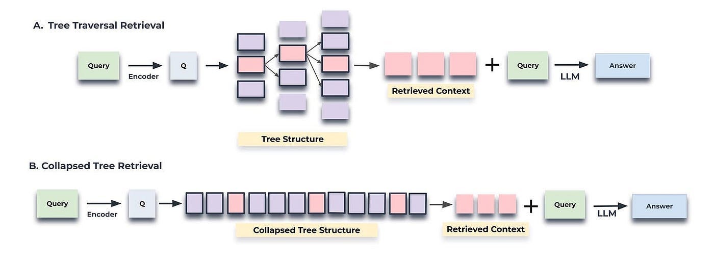
Tree traversal begins at the root level of the tree and retrieves the top-k nodes (in this case, the top-1) based on their cosine similarity to the query vector. At each level, it retrieves the top-k nodes from the children of the previous layer’s top-k nodes, the corresponding code is shown below.
class TreeRetriever(BaseRetriever):
    ...
    ...
    def retrieve_information(
        self, current_nodes: List[Node], query: str, num_layers: int
    ) -> str:
        """
        Retrieves the most relevant information from the tree based on the query.

        Args:
            current_nodes (List[Node]): A List of the current nodes.
            query (str): The query text.
            num_layers (int): The number of layers to traverse.

        Returns:
            str: The context created using the most relevant nodes.
        """

        query_embedding = self.create_embedding(query)

        selected_nodes = []

        node_list = current_nodes

        for layer in range(num_layers):

            embeddings = get_embeddings(node_list, self.context_embedding_model)

            distances = distances_from_embeddings(query_embedding, embeddings)

            indices = indices_of_nearest_neighbors_from_distances(distances)

            if self.selection_mode == "threshold":
                best_indices = [
                    index for index in indices if distances[index] > self.threshold
                ]

            elif self.selection_mode == "top_k":
                best_indices = indices[: self.top_k]

            nodes_to_add = [node_list[idx] for idx in best_indices]

            selected_nodes.extend(nodes_to_add)

            if layer != num_layers - 1:

                child_nodes = []

                for index in best_indices:
                    child_nodes.extend(node_list[index].children)

                # take the unique values
                child_nodes = list(dict.fromkeys(child_nodes))
                node_list = [self.tree.all_nodes[i] for i in child_nodes]

        context = get_text(selected_nodes)
        return selected_nodes, context
In contrast, the collapsed tree condenses the tree into a single layer and retrieves nodes until a threshold number of tokens is reached, again based on cosine similarity to the query vector, the corresponding code is shown below.
class TreeRetriever(BaseRetriever):
    ...
    ...
    def retrieve_information_collapse_tree(self, query: str, top_k: int, max_tokens: int) -> str:
        """
        Retrieves the most relevant information from the tree based on the query.

        Args:
            query (str): The query text.
            max_tokens (int): The maximum number of tokens.

        Returns:
            str: The context created using the most relevant nodes.
        """

        query_embedding = self.create_embedding(query)

        selected_nodes = []

        node_list = get_node_list(self.tree.all_nodes)

        embeddings = get_embeddings(node_list, self.context_embedding_model)

        distances = distances_from_embeddings(query_embedding, embeddings)

        indices = indices_of_nearest_neighbors_from_distances(distances)

        total_tokens = 0
        for idx in indices[:top_k]:

            node = node_list[idx]
            node_tokens = len(self.tokenizer.encode(node.text))

            if total_tokens + node_tokens > max_tokens:
                break

            selected_nodes.append(node)
            total_tokens += node_tokens

        context = get_text(selected_nodes)
        return selected_nodes, context
So which method is better?
RAPTOR made a comparison, as shown in Figure 4.
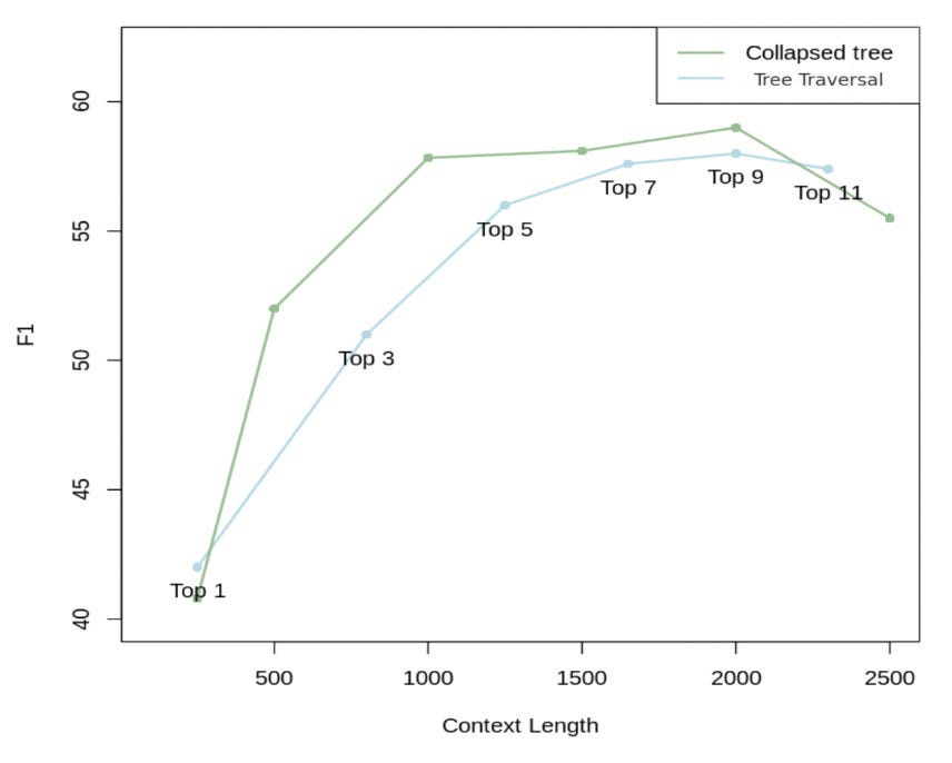
As demonstrated in Figure 4, collapsed tree with 2000 tokens yields the best outcome. This is because it offers more flexibility than tree traversal. Specifically, by simultaneously searching all nodes, it retrieves information at the appropriate granularity level for the given problem.
Figure 5 illustrates how RAPTOR retrieves information for two queries related to the Cinderella story: “What is the central theme of the story?” and “How did Cinderella find a happy ending?”.
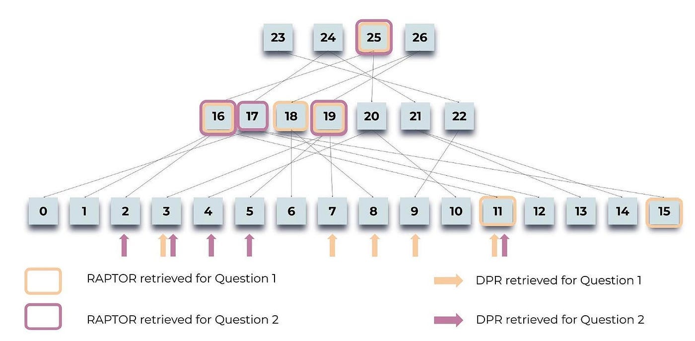
Highlighted nodes indicate RAPTOR’s selections, while arrows point to DPR’s(Dense Passage Retrieval) leaf nodes. Importantly, the context provided by RAPTOR often includes the information retrieved by DPR, either directly or within higher-layer summaries.
Graph RAG
Graph RAG employs LLM to construct a graph-based text index in two stages:
Initially, it derives a knowledge graph from the source documents.
Subsequently, it generates community summaries for all closely connected entity groups.
Given a query, each community summary contributes to a partial response. These partial responses are then aggregated to form the final global answer.
Overview
Figure 6 shows the pipeline of Graph RAG. The purple box signifies the indexing operations, while the green box indicates the query operations.
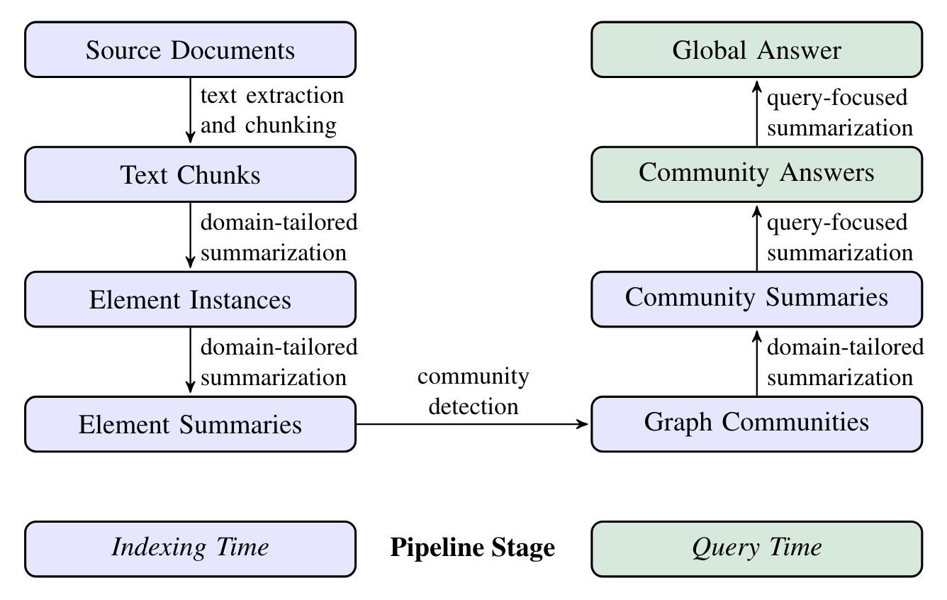
Graph RAG employs LLM prompts specific to the dataset’s domain to detect, extract, and summarize nodes (like entities), edges (like relations), and covariates (like claims).
Community detection is utilized to divide the graph into groups of elements (nodes, edges, covariates) that LLM can summarize at both the time of indexing and querying.
The global answer for a particular query is produced by conducting a final round of query-focused summarization on all community summaries associated with that query.
The implementation of each step in Figure 6 will be explained below. It’s worth noting that as of June 12, 2024, Graph RAG is not currently open source, so it can’t be discussed in relation to the source code.
Step 1 : Source Documents → Text Chunks
The trade-off of chunk size is a longstanding problem for RAG.
If the chunk is too long, the number of LLM calls decreases. However, due to the constraints of the context window, it becomes challenging to fully comprehend and manage large amounts of information. This situation can lead to a decline in the recall rate.
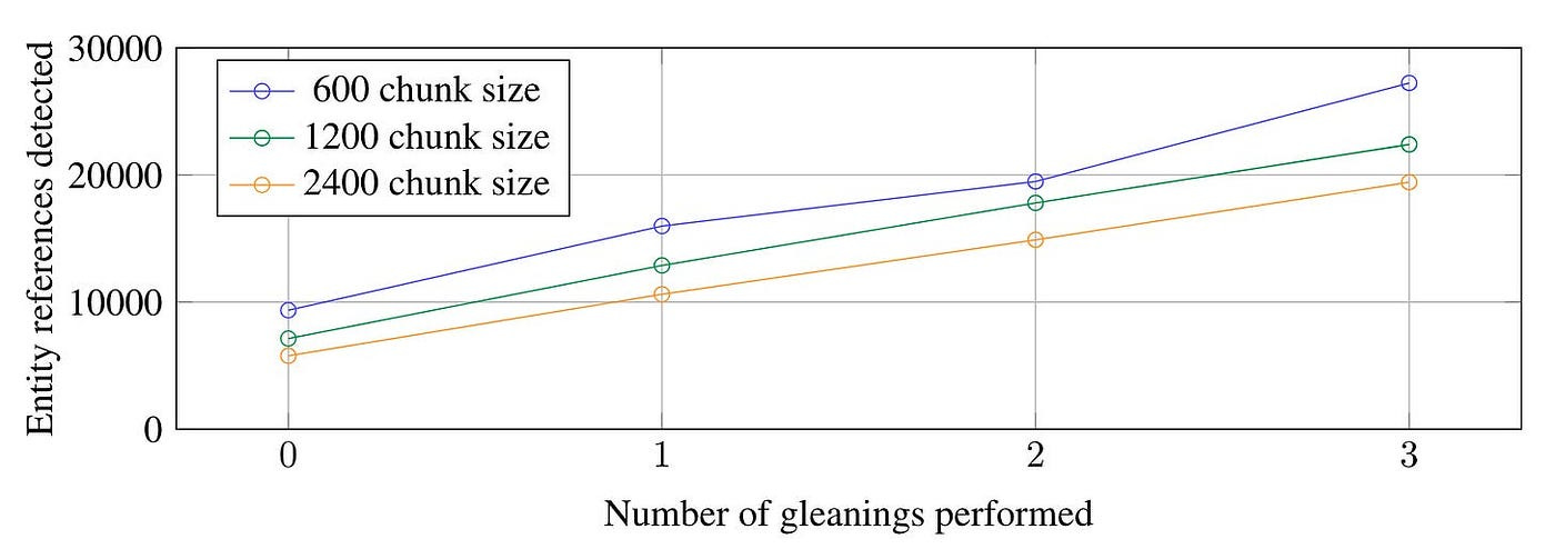
As illustrated in Figure 7, for the HotPotQA dataset, a chunk size of 600 tokens extracts twice as many effective entities compared to a chunk size of 2400 tokens.
Step 2: Text Chunks → Element Instances (Entities and Relationships)
The method involves constructing a knowledge graph by extracting entities and their relationships from each chunk. This is achieved through the combination of LLMs and prompt engineering.
Simultaneously, Graph RAG employs a multi-stage iterative process. This process requires the LLM to determine if all entities have been extracted, similar to a binary classification problem.
Step 3: Element Instances → Element Summaries → Graph Communities → Community Summaries
In the previous step, the extracting entities, relationships, and claims is actually a form of abstractive summarization.
However, Graph RAG believes that this is not sufficient and that further summarizations of these “elements” are required using LLMs.
A potential concern is that LLMs may not always extract references to the same entity in the same text format. This could lead to duplicate entity elements, consequently generating duplicate nodes in the graph.
This concern will quickly dissipate.
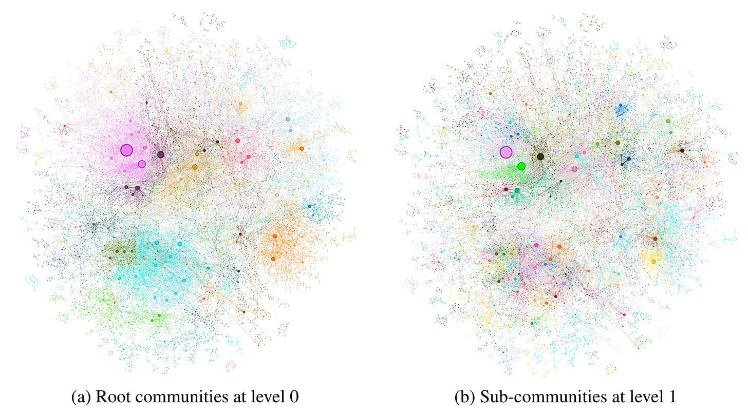
Graph RAG employs community detection algorithms to identify community structures within the graph, incorporating closely linked entities into the same community. Figure 8 presents the graph communities identified in the MultiHop-RAG dataset using Leiden algorithm.
In this scenario, even if LLM fails to identify all variants of an entity consistently during extraction, community detection can help establish the connections between these variants. Once grouped into a community, it signifies that these variants refer to the same entity connotation, just with different expressions or synonyms. This is akin to entity disambiguation in the field of knowledge graph.

After identifying the community, we can generate report-like summaries for each community within the Leiden hierarchy. These summaries are independently useful in understanding the global structure and semantics of the dataset. They can also be used to comprehend the corpus without any problems.
Figure 9 shows the generation method of community summary.
Step 4: Community Summaries → Community Answers → Global Answer
We’ve now reached the final step: generating the final answer based on the community summary from the previous step.
Due to the hierarchical nature of community structure, summaries from different levels can answer various questions.
However, this brings us to another question: with multiple levels of community summaries available, which level can strike a balance between detail and coverage?
Graph RAG, upon further evaluation(section 3 in the paper of Graph RAG), selects the most suitable level of abstraction.
For a given community level, the global answer to any user query is generated, as shown in Figure 10.

HippoRAG
HippoRAG is a novel retrieval framework, taking inspiration from hippocampal indexing theory of human long-term memory. It collaborates with LLMs, knowledge graphs, and personalized PageRank algorithms. This collaboration mimics the varied roles of the neocortex and hippocampus in human memory.
Key Idea
Figure 11 illustrates how the human brain can relatively easily tackle difficult tasks of knowledge integration.
The Hippocampal Memory Indexing Theory, a well-known theory of human long-term memory, offers a possible explanation for this remarkable capability.
Specifically, the environment-based, continually updated memory relies on the interaction between the neocortex and the C-shaped hippocampus. The neocortex processes and stores the actual memory representation, while the hippocampus maintains the hippocampal index. This index is a set of interconnected indexes that point to memory units in the neocortex and store their associations.
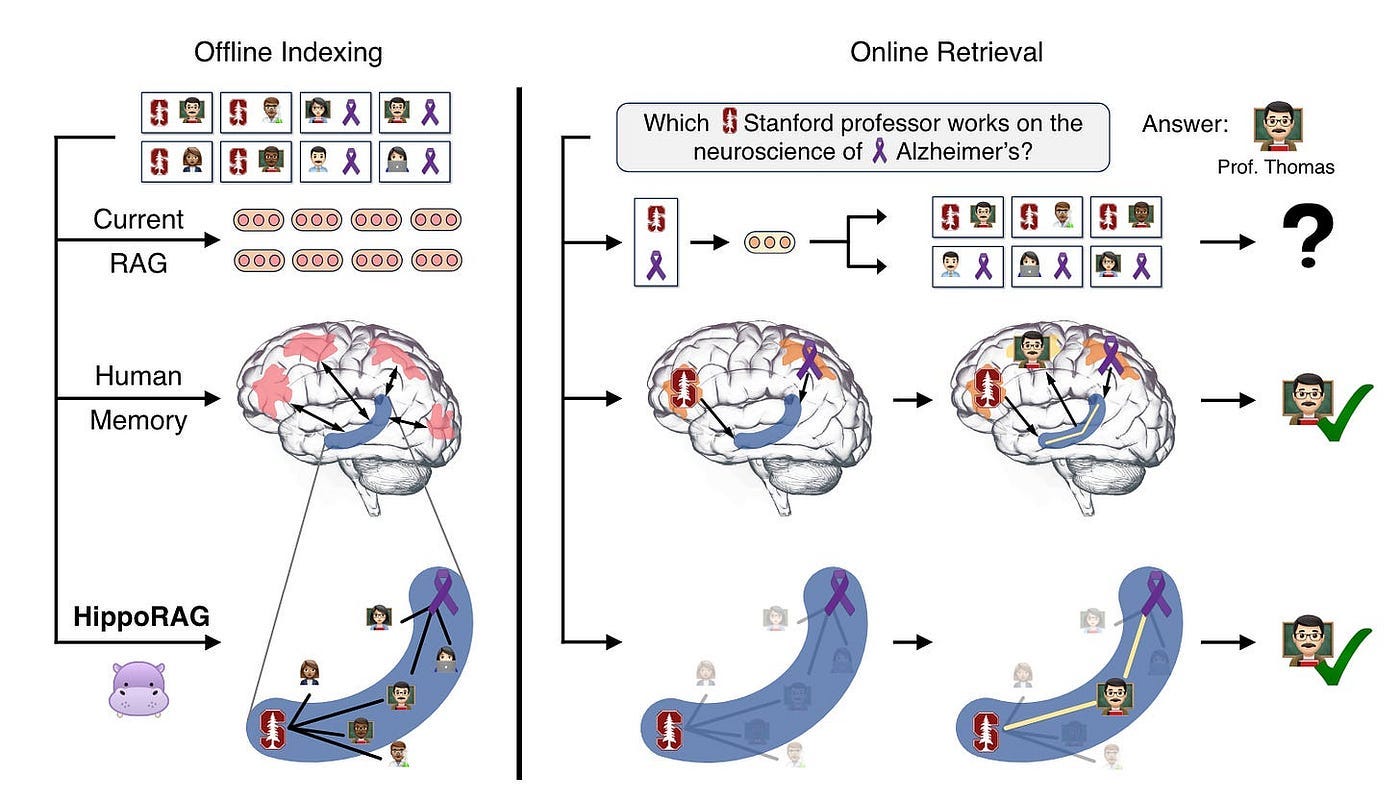
In Figure 11, we aim to identify a Stanford professor involved in Alzheimer’s disease research from numerous passages potentially describing thousands of Stanford professors and Alzheimer’s disease researchers.
Traditional RAG, which encode passages independently, struggle to identify Professor Thomas unless a passage simultaneously mentions these two features.
In contrast, people familiar with this professor could quickly remember him, thanks to our brains’ associative memory capabilities, believed to be driven by the C-shaped hippocampal index structure shown in blue in Figure 11.
Inspired by this mechanism, HippoRAG enables LLMs to construct and utilize similar association maps to manage knowledge integration tasks.
Overview
Inspired by Figure 11, each component of HippoRAG corresponds to one of the three components of human long-term memory, as shown in Figure 12.
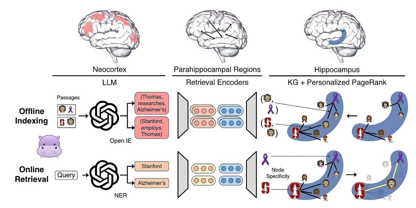
HippoRAG simulates the three components of human long-term memory to emulate its pattern separation and completion functions.
For offline indexing, LLM processes passages into open KG triples. These are then added to artificial hippocampal index, while synthetic parahippocampal regions (PHR) detect synonyms. In the above example, HippoRAG extracts triples involving Professor Thomas and incorporates them into the KG.
For online retrieval, LLM neocortex extracts named entities from queries. Parahippocampal retrieval encoders then link them to hippocampal index. HippoRAG utilizes a personalized PageRank algorithm for context-based retrieval and extracts information related to Professor Thomas.
Overall Process Demonstration
Here is a practical example that introduces the pipeline of HippoRAG.
Figure 13 displays the question, its answer, and its supporting and distractor passages.
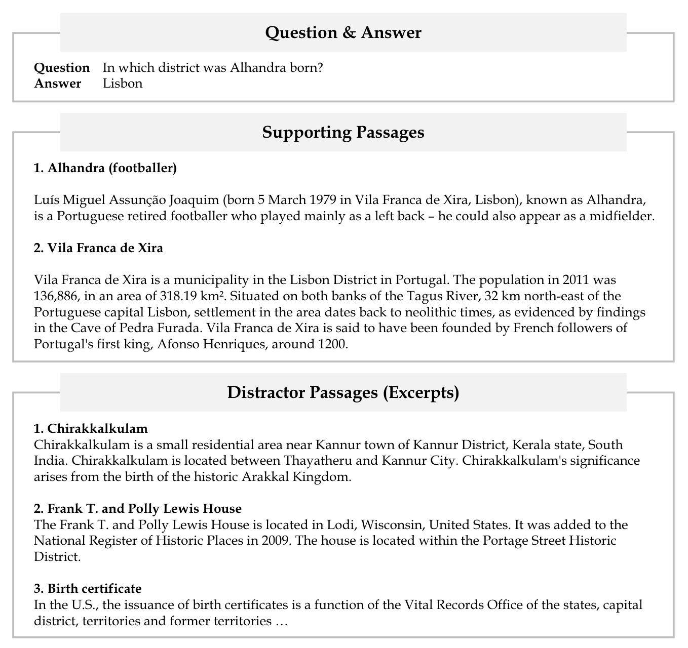
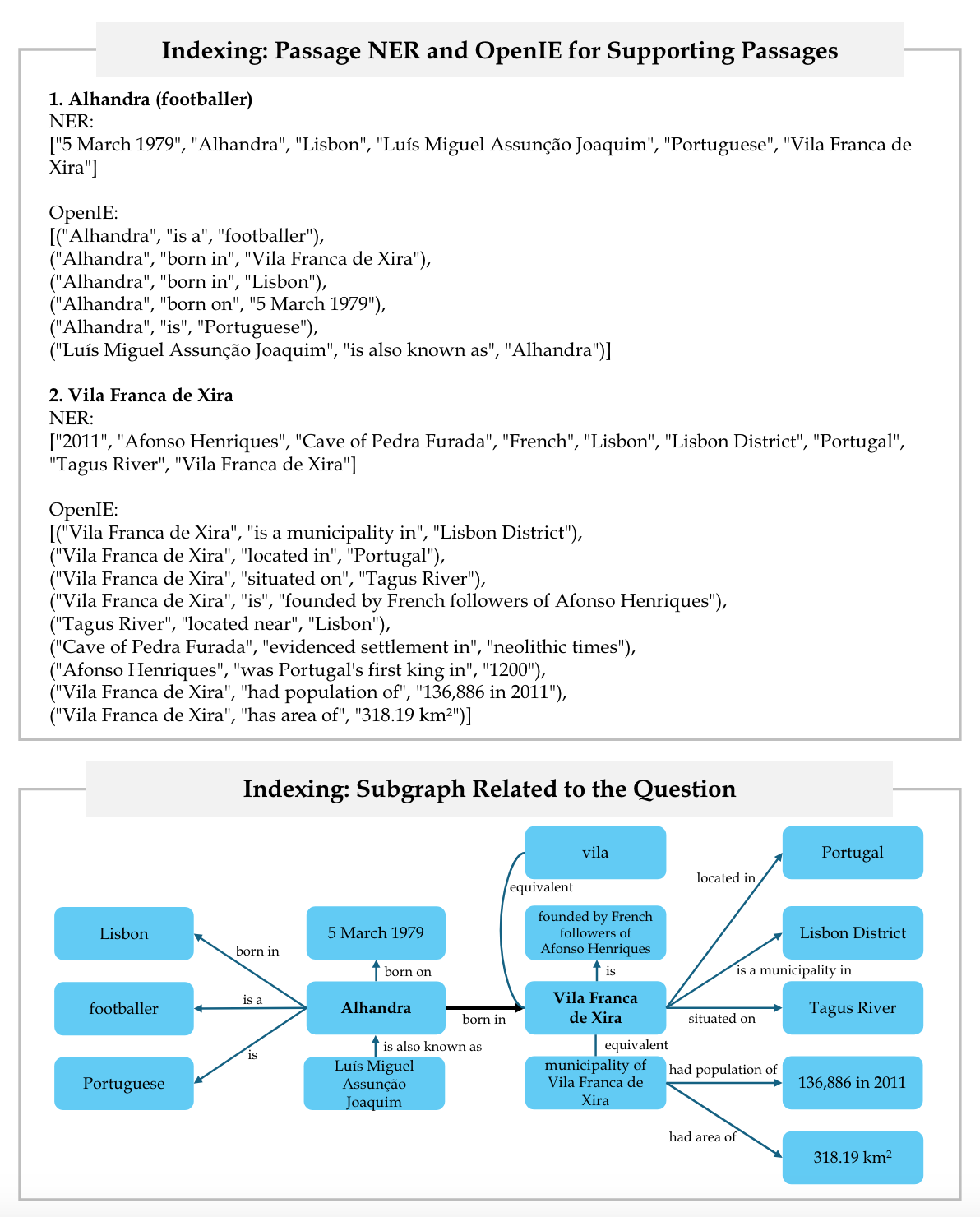
Figure 14 depicts the indexing stage, including the OpenIE procedure and the relevant subgraph of knowledge graph.
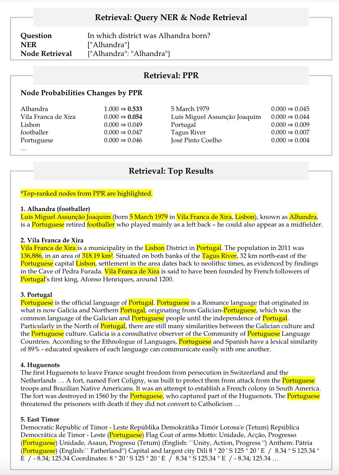
Lastly, Figure 15 demonstrates the retrieval stage, showcasing query Named Entity Recognition (NER), query node retrieval, the impact of the Personalized Page Rank (PPR) algorithm on node probabilities, and the computation of the top retrieval results.
Below, combined with the source code, we specifically discuss how HippoRAG builds long-term memory and how to retrieve it in two aspects.
How to Build Long-Term Memory
The process of building long-term memory primarily consists of the following three steps.
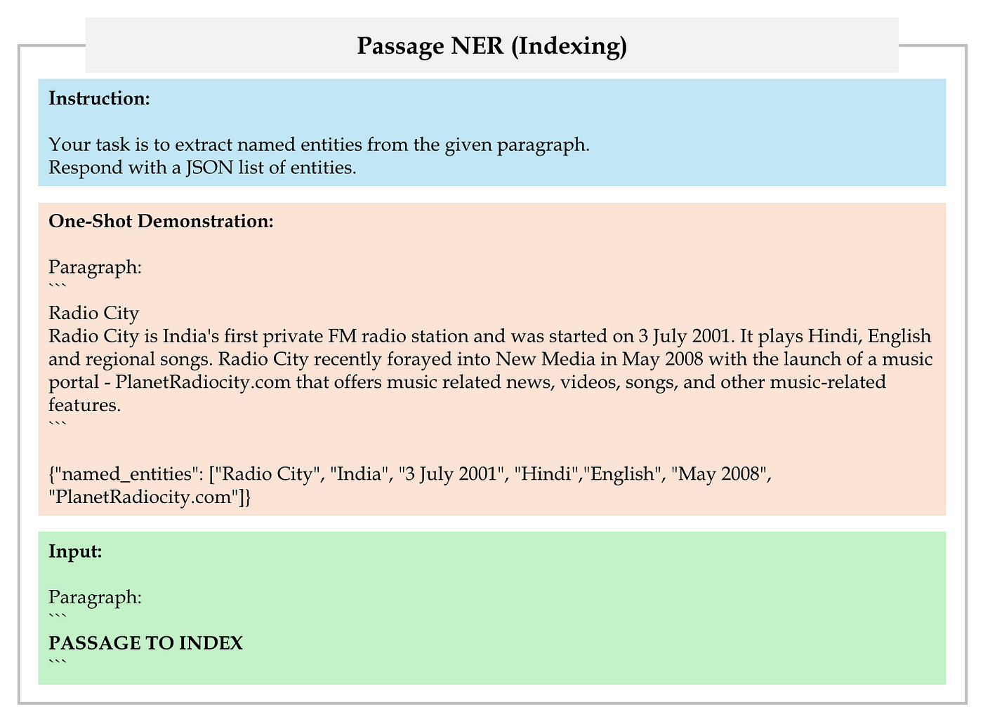
First, employ LLM to extract a set of named entities from each passage in retrieval corpus using OpenIE, as depicted in Figure 16.
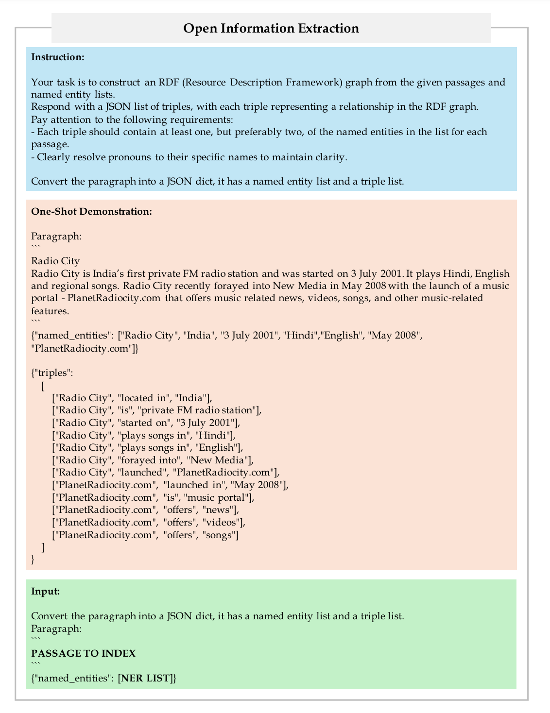
Next, add the named entities to the OpenIE prompts to extract the final triples, as depicted in Figure 17.
Finally, utilize the fine-tuned, off-the-shelf dense encoder to create knowledge graph, which will also be used for retrieval.
How to Retrieve
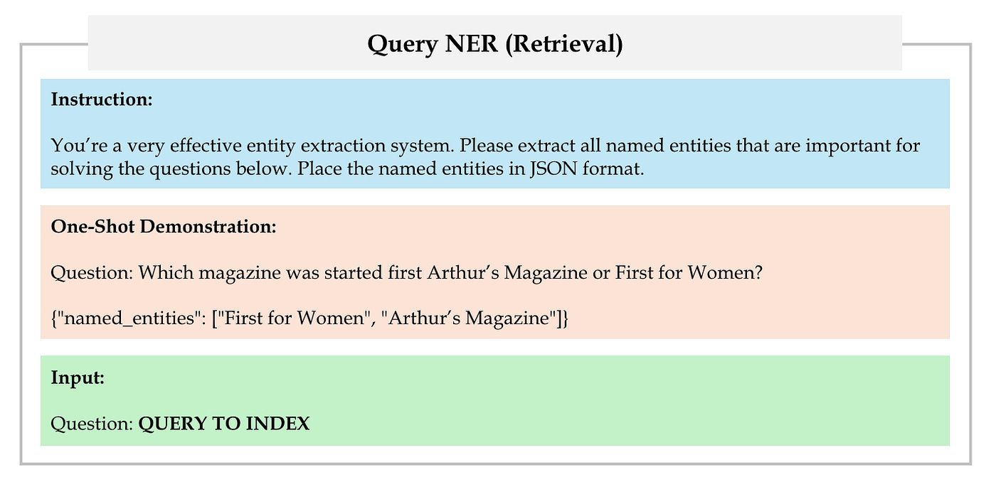
First, employ LLM to extract a set of named entities from user query, as shown in Figure 18.
Then, link these named entities to nodes in the knowledge graph based on the similarity determined by the retrieval encoder. We refer to these selected nodes as query nodes.
In the hippocampus, neural pathways between elements of the hippocampal index enable relevant neighborhoods to become activated and recalled upstream.
To imitate this efficient graph search process, HippoRAG leverages the Personalized PageRank (PPR) algorithm, a version of PageRank that distributes probability across a graph only through a set of user-defined source nodes. The corresponding code is shown below.
    def rank_docs(self, query: str, top_k=10):
        """
        Rank documents based on the query
        @param query: the input phrase
        @param top_k: the number of documents to return
        @return: the ranked document ids and their scores
        """
        ...
        ...
        # Run Personalized PageRank (PPR) or other Graph Alg Doc Scores
        if len(query_ner_list) > 0:
            combined_vector = np.max([top_phrase_vectors], axis=0)

            if self.graph_alg == 'ppr':
                ppr_phrase_probs = self.run_pagerank_igraph_chunk([top_phrase_vectors])[0]
            elif self.graph_alg == 'none':
                ppr_phrase_probs = combined_vector
            elif self.graph_alg == 'neighbor_2':
                ppr_phrase_probs = self.get_neighbors(combined_vector, 2)
            elif self.graph_alg == 'neighbor_3':
                ppr_phrase_probs = self.get_neighbors(combined_vector, 3)
            elif self.graph_alg == 'paths':
                ppr_phrase_probs = self.get_neighbors(combined_vector, 3)
            else:
                assert False, f'Graph Algorithm {self.graph_alg} Not Implemented'

            fact_prob = self.facts_to_phrases_mat.dot(ppr_phrase_probs)
            ppr_doc_prob = self.docs_to_facts_mat.dot(fact_prob)
            ppr_doc_prob = min_max_normalize(ppr_doc_prob)
        else:
            ppr_doc_prob = np.ones(len(self.extracted_triples)) / len(self.extracted_triples)
        ...
        ...
Finally, as is done when the hippocampal signal is sent upstream, HippoRAG aggregates the output PPR node probability over the previously indexed passages and uses that to rank them for retrieval.
spRAG
spRAG is a method for managing complex queries. It enhances the performance of standard RAG through two key techniques:
AutoContext
Relevant Segment Extraction (RSE)
We focus on how spRAG handles complex queries across chunks. It’s worth noting that there are currently no papers on spRAG, only analysis combined with code.
AutoContext: Automatic Injection of Document-Level Context
In traditional RAG, documents are typically divided into fixed-length chunks for embedding. This simple method often overlooks document-level context information, leading to less accurate and comprehensive context embedding.
To address this issue, AutoContext was developed. Its key idea is to automatically incorporate document-level context information into each chunk before embedding.
Specifically, it creates a document summary of 1–2 sentences and adds it, along with the filename, to the start of each chunk. As a result, each chunk is no longer isolated but carries the context information of the entire document. The code for getting document summary is shown below.
def get_document_context(auto_context_model: LLM, text: str, document_title: str, auto_context_guidance: str = ""):
    # truncate the content if it's too long
    max_content_tokens = 6000 # if this number changes, also update the truncation message above
    text, num_tokens = truncate_content(text, max_content_tokens)
    if num_tokens < max_content_tokens:
        truncation_message = ""
    else:
        truncation_message = TRUNCATION_MESSAGE

    # get document context
    prompt = PROMPT.format(auto_context_guidance=auto_context_guidance, document=text, document_title=document_title, truncation_message=truncation_message)
    chat_messages = [{"role": "user", "content": prompt}]
    document_context = auto_context_model.make_llm_call(chat_messages)
    return document_context
Relevant Segment Extraction: Intelligent Combination of Related Text chunks
RSE is a post-processing step. Its objective is to intelligently identify and combine chunks that can provide the most relevant information, thereby forming longer segments.
Specifically, RSE first groups the retrieved chunks that are either content-similar or semantically related. Then, based on the query requirements, it intelligently selects and combines these chunks to form the best segments. The corresponding code is shown below.
def get_best_segments(all_relevance_values: list[list], document_splits: list[int], max_length: int, overall_max_length: int, minimum_value: float) -> list[tuple]:
    """
    This function takes the chunk relevance values and then runs an optimization algorithm to find the best segments.

    - all_relevance_values: a list of lists of relevance values for each chunk of a meta-document, with each outer list representing a query
    - document_splits: a list of indices that represent the start of each document - best segments will not overlap with these

    Returns
    - best_segments: a list of tuples (start, end) that represent the indices of the best segments (the end index is non-inclusive) in the meta-document
    """
    best_segments = []
    total_length = 0
    rv_index = 0
    bad_rv_indices = []
    while total_length < overall_max_length:
        # cycle through the queries
        if rv_index >= len(all_relevance_values):
            rv_index = 0
        # if none of the queries have any more valid segments, we're done
        if len(bad_rv_indices) >= len(all_relevance_values):
            break
        # check if we've already determined that there are no more valid segments for this query - if so, skip it
        if rv_index in bad_rv_indices:
            rv_index += 1
            continue

        # find the best remaining segment for this query
        relevance_values = all_relevance_values[rv_index] # get the relevance values for this query
        best_segment = None
        best_value = -1000
        for start in range(len(relevance_values)):
            # skip over negative value starting points
            if relevance_values[start] < 0:
                continue
            for end in range(start+1, min(start+max_length+1, len(relevance_values)+1)):
                # skip over negative value ending points
                if relevance_values[end-1] < 0:
                    continue
                # check if this segment overlaps with any of the best segments
                if any(start < seg_end and end > seg_start for seg_start, seg_end in best_segments):
                    continue
                # check if this segment overlaps with any of the document splits
                if any(start < split and end > split for split in document_splits):
                    continue
                # check if this segment would push us over the overall max length
                if total_length + end - start > overall_max_length:
                    continue
                segment_value = sum(relevance_values[start:end]) # define segment value as the sum of the relevance values of its chunks
                if segment_value > best_value:
                    best_value = segment_value
                    best_segment = (start, end)

        # if we didn't find a valid segment, mark this query as done
        if best_segment is None or best_value < minimum_value:
            bad_rv_indices.append(rv_index)
            rv_index += 1
            continue

        # otherwise, add the segment to the list of best segments
        best_segments.append(best_segment)
        total_length += best_segment[1] - best_segment[0]
        rv_index += 1

    return best_segments
Insights and Thoughts
Comparison of Algorithms and Data Structures
RAPTOR constructs a tree-like data structure through clustering and performs retrieval based on this structure.
Though both Graph RAG and HippoRAG employ knowledge graphs, they have some differences:
Regarding data structure, Graph RAG incorporates information by summarizing knowledge elements. Therefore, the summarization process needs to be repeated anytime new data is added. This is also true for RAPTOR. Conversely, HippoRAG can seamlessly integrate new knowledge by merely adding edges to its knowledge graph.
In the context of retrieval algorithms, Graph RAG depends on community detection, whereas HippoRAG utilizes the Personalized PageRank (PPR) algorithm.
Unlike the others, spRAG doesn’t use advanced data structures. It simply adds the document summary and filename to each chunk, proceeding to perform retrieval based on relevance values. This also suggests that the indexing and query speed of spRAG should be the fastest.
About Performance
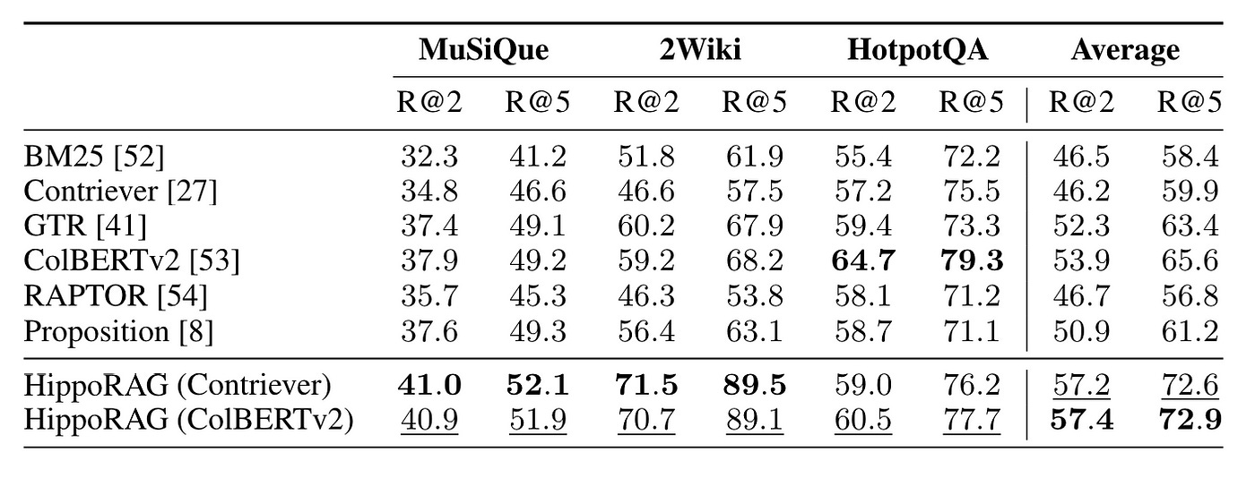
HippoRAG conducted experiments using RAPTOR as the baseline, demonstrating some results that surpassed those of RAPTOR, as shown in Figure 19.
In the Graph RAG paper, performance comparison experiments are not included.
Additionally, at present, there is no paper available on spRAG.
About the Enhanced Range
The four methods — RAPTOR, Graph RAG, HippoRAG, and spRAG — aim to enhance the understanding of the entire corpus.
They each build data structures based on the entire corpus.
About Customizability
In this context, HippoRAG outperforms because all of its components are off-the-shelf, eliminating the need for additional training, as shown in Figure 20.
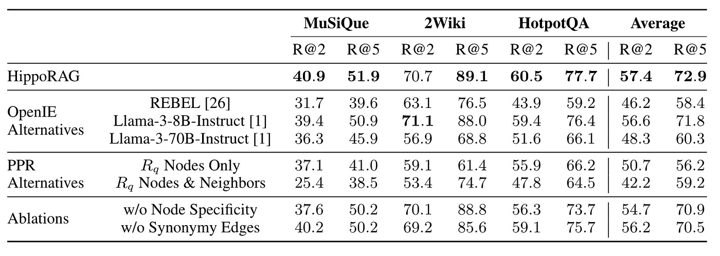
Thus, by fine-tuning specific components, there’s significant potential for improvement.
Conclusion
This article introduces four new methods to enhance the global comprehension of traditional RAG for documents or corpora, supplemented by code explanations. It also includes my insights and thoughts.
If you’re interested in RAG, feel free to check out my other articles.
Lastly, if there are any errors or omissions, or if you have any thoughts to share, please feel free to discuss in the comments section.

