
A Detailed Explanation of Mixtral 8x7B Model
Including principles, diagrams, and code analysis.

Since the end of 2023, the Mixtral 8x7B[1] has become a highly popular model in the field of large language models. It has gained this popularity because it outperforms the Llama2 70B model with fewer parameters (less than 8x7B) and computations (less than 2x7B), and even exceeds the capabilities of GPT-3.5 in certain aspects.
This article primarily focuses on the code and includes illustrations to explain the principles behind the Mixtral model.
Overall Architecture
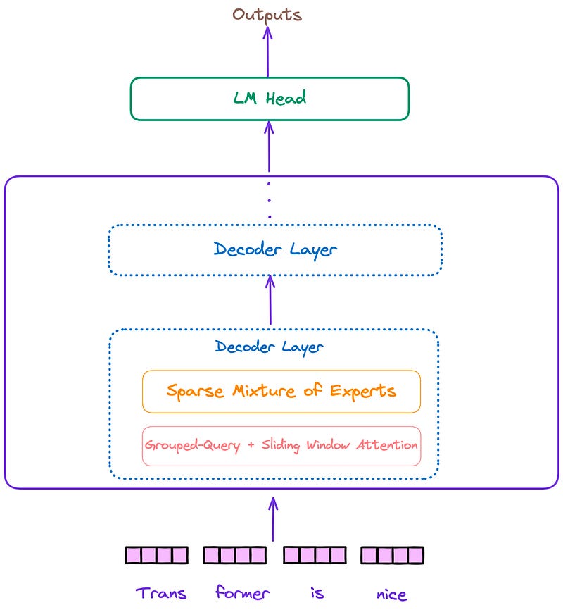
The overall architecture of the Mixtral model, similar to Llama and other decoder-only models, can be divided into three parts: the input embedding layer, several decoder blocks, and the language model decoding head. This is illustrated in Figure 1.
Decoder Layer
The architecture of the decoder layer is depicted in Figure 2. Each decoder layer mainly consists of two modules: attention and a sparse mixture of experts(SMoE).
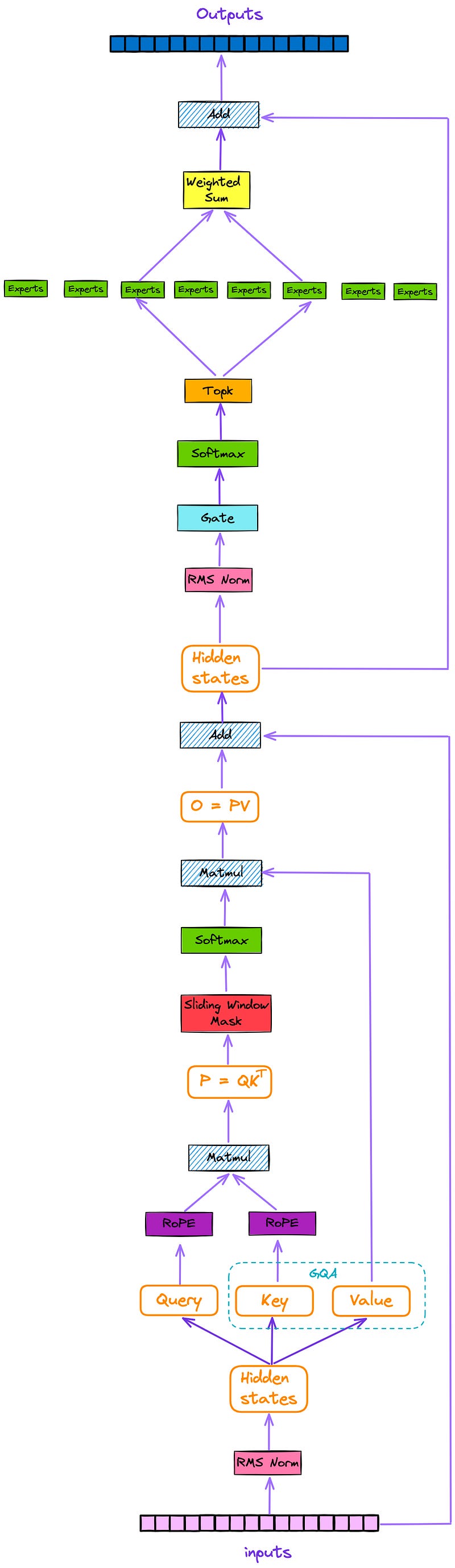
We can see that the Mixtral model incorporates additional features, such as a sparse mixture of experts(SMoE), Sliding Window Attention(SWA), Grouped-Query Attention(GQA), and Rotary Position Embedding (RoPE).
Next, this article will explain these important features.
Sparse Mixture of Experts (SMoE)
From Figure 1 and Figure 2, we already know the position of SMoE in the entire model architecture. In this section, let’s take a closer look at the internal structure of SMoE. Here, the SMoE module is extracted separately, as shown in Figure 3.
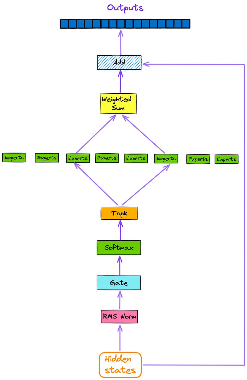
As depicted in Figure 3, every token that is inputted into the model is subsequently directed (via Gating or Router) to top k experts(by default, k = 2) after going through the attention layer and residual connections.
The outputs of the most relevant experts are then weighted and summed, and subsequently passed through a residual connection to obtain the outputs of the current decoder layer.
First, let’s take a look at the code of the expert:
class MixtralBLockSparseTop2MLP(nn.Module):
    def __init__(self, config: MixtralConfig):
        super().__init__()
        self.ffn_dim = config.intermediate_size
        self.hidden_dim = config.hidden_size

        self.w1 = nn.Linear(self.hidden_dim, self.ffn_dim, bias=False)
        self.w2 = nn.Linear(self.ffn_dim, self.hidden_dim, bias=False)
        self.w3 = nn.Linear(self.hidden_dim, self.ffn_dim, bias=False)

        self.act_fn = ACT2FN[config.hidden_act]

    def forward(self, hidden_states, routing_weights):
        current_hidden_states = self.act_fn(self.w1(hidden_states)) * self.w3(hidden_states)
        current_hidden_states = self.w2(current_hidden_states)
        return routing_weights * current_hidden_states
Once we have an expert, MixtralSparseMoeBlock combines a default of 8 experts together (self.num_experts = 8). The gate layer selects the top 2( by default k = 2) expert models for computation for each token. You can find the code for this here.
class MixtralSparseMoeBlock(nn.Module):
    """
    This implementation is
    strictly equivalent to standard MoE with full capacity (no
    dropped tokens). It's faster since it formulates MoE operations
    in terms of block-sparse operations to accomodate imbalanced
    assignments of tokens to experts, whereas standard MoE either
    (1) drop tokens at the cost of reduced performance or (2) set
    capacity factor to number of experts and thus waste computation
    and memory on padding.
    """

    def __init__(self, config):
        super().__init__()
        self.hidden_dim = config.hidden_size
        self.ffn_dim = config.intermediate_size
        self.num_experts = config.num_local_experts
        self.top_k = config.num_experts_per_tok

        # gating
        self.gate = nn.Linear(self.hidden_dim, self.num_experts, bias=False)
        # Experts
        self.experts = nn.ModuleList([MixtralBLockSparseTop2MLP(config) for _ in range(self.num_experts)])

    def forward(self, hidden_states: torch.Tensor) -> torch.Tensor:
        """ """
        batch_size, sequence_length, hidden_dim = hidden_states.shape
        hidden_states = hidden_states.view(-1, hidden_dim)
        # router_logits: (batch * sequence_length, n_experts)
        # Retrieve the scores provided by each expert,
        # with the dimensions of batch * sequence * num_experts,
        # and then select the topk experts.
        router_logits = self.gate(hidden_states)

        routing_weights = F.softmax(router_logits, dim=1, dtype=torch.float)
        routing_weights, selected_experts = torch.topk(routing_weights, self.top_k, dim=-1)

        # After obtaining the scores of the top k experts,
        # it is necessary to normalize them again.
        # This step is important to assign appropriate weights to
        # the results calculated for the subsequent experts
        routing_weights /= routing_weights.sum(dim=-1, keepdim=True)
        # we cast back to the input dtype
        routing_weights = routing_weights.to(hidden_states.dtype)

        final_hidden_states = torch.zeros(
            (batch_size * sequence_length, hidden_dim), dtype=hidden_states.dtype, device=hidden_states.device
        )

        # One hot encode the selected experts to create an expert mask
        # this will be used to easily index which expert is going to be sollicitated
        expert_mask = torch.nn.functional.one_hot(selected_experts, num_classes=self.num_experts).permute(2, 1, 0)

        # Loop over all available experts in the model and perform the computation on each expert
        for expert_idx in range(self.num_experts):
            # Choose the expert you are currently using
            expert_layer = self.experts[expert_idx]
            # Select the index corresponding to the current expert
            # top_x actually corresponds to the current expert's token index.
            idx, top_x = torch.where(expert_mask[expert_idx])

            if top_x.shape[0] == 0:
                continue

            # in torch it is faster to index using lists than torch tensors
            top_x_list = top_x.tolist()
            idx_list = idx.tolist()

            # Index the correct hidden states and compute the expert hidden state for
            # the current expert. We need to make sure to multiply the output hidden
            # states by `routing_weights` on the corresponding tokens (top-1 and top-2)
            current_state = hidden_states[None, top_x_list].reshape(-1, hidden_dim)
            # The expert model will use selected states to perform
            # calculations and multiply them by the weight
            current_hidden_states = expert_layer(current_state, routing_weights[top_x_list, idx_list, None])

            # However `index_add_` only support torch tensors for indexing so we'll use
            # the `top_x` tensor here.
            # Add the output of each expert to the final result according to their index.
            final_hidden_states.index_add_(0, top_x, current_hidden_states.to(hidden_states.dtype))
        final_hidden_states = final_hidden_states.reshape(batch_size, sequence_length, hidden_dim)
        return final_hidden_states, router_logits
To enhance comprehension, I have added some comments within the code.
The above code can be divided into 3 main steps:
For inputs, the gate layer is used to obtain routing information. After normalizing the routing information using softmax, the top
kweights and indices of the experts are selected. The indices are then converted into a sparse matrix calledexpert_mask.Iterate over all experts and perform the following operation: select experts, and each expert only needs to process its own tokens.
To obtain the outputs, calculate the weighted summation of the chosen expert’s output.
Sliding Window Attention(SWA)
In traditional self-attention mechanisms, each token in the sequence interacts with every other token, resulting in a time and space complexity of O(n²), where n is the input sequence length, as shown in Figure 4(a). Once we need to process longer texts, it will result in a significant computational burden.

So, in order to solve this dilemma and enable Transformer to be used for longer texts, Longformer[2] proposes the following sliding window attention mechanism.
As shown in Figure 4(b), for a token in the sequence, the sliding window attention sets a fixed-size sliding window, denoted as w. It specifies that each token in the sequence can only attend to w tokens, with w/2 tokens on each side. Self-attention is performed within this window. This reduces the time complexity from O(n²) to O(n * w).
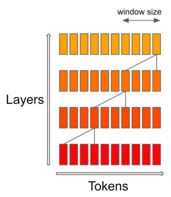
Furthermore, we do not need to worry about this setting not being able to capture the semantic information of the entire sequence. This is because the transformer model itself is a stacked structure, with higher layers having a wider receptive field compared to lower layers. Naturally, it is able to see more information and has the capability to model and integrate the global representation of the entire sequence, similar to CNN. For a transformer model with L layers, the receptive field size at the top layer is L * w, as shown in Figure 5:
Below is the code for generating the attention mask in Mixtral:
@dataclass
class AttentionMaskConverter:

    ...
    ...

    @staticmethod
    def _make_causal_mask(
        input_ids_shape: torch.Size,
        dtype: torch.dtype,
        device: torch.device,
        past_key_values_length: int = 0,
        sliding_window: Optional[int] = None,
    ):
        """
        Make causal mask used for bi-directional self-attention.
        """
        bsz, tgt_len = input_ids_shape
        mask = torch.full((tgt_len, tgt_len), torch.finfo(dtype).min, device=device)
        mask_cond = torch.arange(mask.size(-1), device=device)
        mask.masked_fill_(mask_cond < (mask_cond + 1).view(mask.size(-1), 1), 0)

        mask = mask.to(dtype)

        if past_key_values_length > 0:
            mask = torch.cat([torch.zeros(tgt_len, past_key_values_length, dtype=dtype, device=device), mask], dim=-1)

        # add lower triangular sliding window mask if necessary
        if sliding_window is not None:
            diagonal = past_key_values_length - sliding_window + 1

            context_mask = 1 - torch.triu(torch.ones_like(mask, dtype=torch.int), diagonal=diagonal)
            mask.masked_fill_(context_mask.bool(), torch.finfo(dtype).min)

        return mask[None, None, :, :].expand(bsz, 1, tgt_len, tgt_len + past_key_values_length)
Rotary Position Embedding (RoPE)
Rotary Position Embedding (RoPE) is a popular positional encoding technique used in many large language models. It effectively incorporates the concept of rotating vectors for position encoding and is implemented using operations of complex numbers.
For more information and code analysis, please refer to

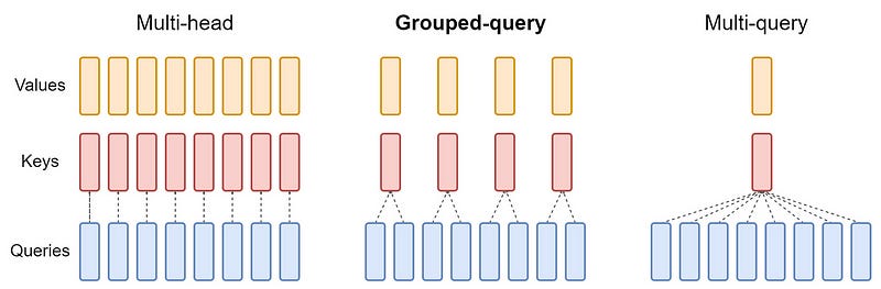
Grouped-Query Attention(GQA)
GQA[4] can be seen as an intermediate or generalized form of multi-query attention(MQA) and multi-head attention(MHA):
When there is only one group in GQA, it is referred to as MQA.
When the number of groups in GQA is equal to the number of attention heads, it is referred to as MHA.
Figure 6 provides a clear visualization of this relationship.
For more information and code analysis, please refer to

Conclusion
Mixtral-8x7B is the first proven effective open-source MoE LLM. It demonstrates that MoE can be successfully implemented and outperforms Dense models with the same activation values.
MoE is a highly promising research direction, and we anticipate further advancements in this field in the future.
Lastly, if there are any errors or omissions in this article, please kindly point them out.
References
[1]: Mistral AI team. Mixtral of experts (2023). URL: https://mistral.ai/news/mixtral-of-experts/.
[2]: I. Beltagy, M. Peters, A. Cohan. Longformer: The Long-Document Transformer(2020). arXiv preprint arXiv:2004.05150.
[3]: Mistral AI team. Mistral Transformer (2023). URL: https://github.com/mistralai/mistral-src.
[4]: J. Ainslie, J. Lee-Thorp, M. Jong, Y. Zemlyanskiy, F. Lebrón, S. Sanghai. GQA: Training Generalized Multi-Query Transformer Models from Multi-Head Checkpoints (2023). arXiv preprint arXiv:2305.13245.